Abstract
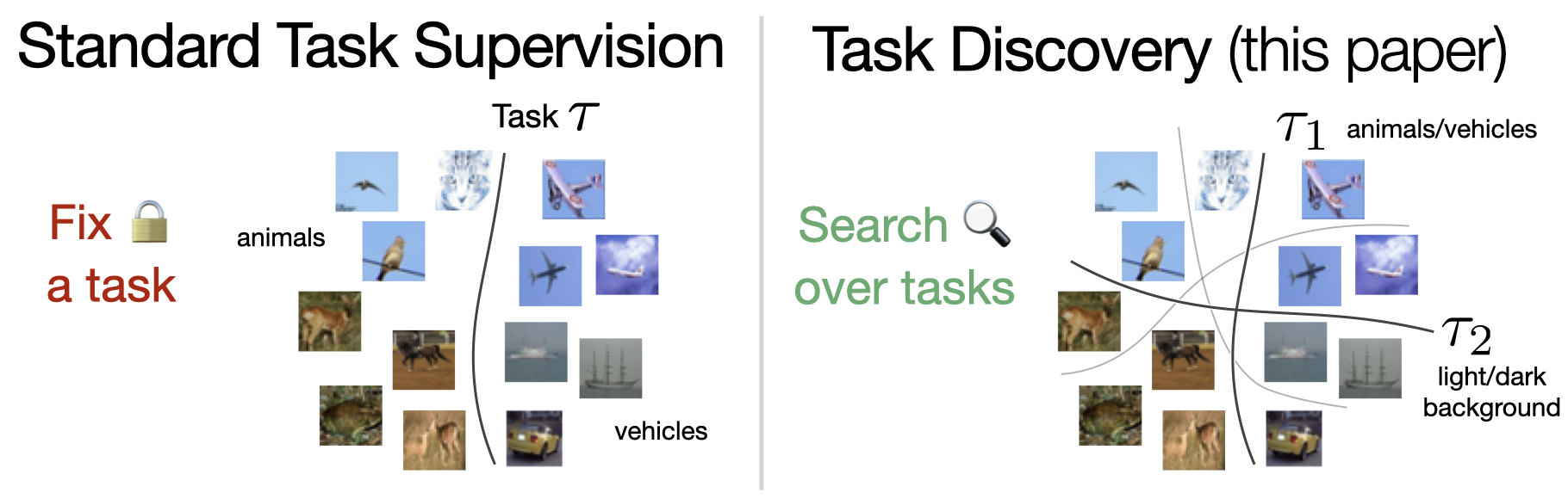
When developing deep learning models, we usually decide what task we want to solve then search for a model that generalizes well on the task. An intriguing question would be: what if, instead of fixing the task and searching in the model space, we fix the model and search in the task space? Can we find tasks that the model generalizes on? How do they look, or do they indicate anything? These are the questions we address in this paper.
We propose a task discovery framework that automatically finds examples of such tasks via optimizing a generalization-based quantity called agreement score. We demonstrate that one set of images can give rise to many tasks on which neural networks generalize well. These tasks are a reflection of the inductive biases of the learning framework and the statistical patterns present in the data, thus they can make a useful tool for analysing the neural networks and their biases. As an example, we show that the discovered tasks can be used to automatically create adversarial train-test splits which make a model fail at test time, without changing the pixels or labels, but by only selecting how the datapoints should be split between the train and test sets. We end with a discussion on human-interpretability of the discovered tasks.
Overview
Task Discovery
We define a task \(\tau\) to be a binary classification of a given set of images \(X\), i.e., \(\tau:X \to \{0, 1\}\) (the multi-class extension is straightforward). Let us consider the following two examples: a human-labelled and a random-labelled tasks over the same set of CIFAR-10 images:
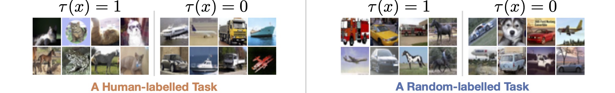
Different tasks defined on the same CIFAR-10 images. The human-labelled task corresponds to a semantic classification defined by humans (animals vs. vehicles in this case). For random-labelled task, each label is assigned randomly and independent of the image content.
We know that a deep enough network, e.g., ResNet-18, can successfully fit any of these tasks to zero train error (Zhang C. et al.). However, it generalizes to new test images only in the case of human-labelled tasks. What does this mean? Generalization is measured as test error w.r.t. to some ground truth labels of the test images. In the case of random-labelled tasks, we can could simply say that the network's test predictions are the ground truth labels and, hence, the test error is zero. The problem, however, is that when we train another network (e.g., from a different initialization) on the same task, it will (as we observe empirically) give different predictions, and the test error will be high. That is, networks trained on the random-labelled task make different predictions on test data, and there is no single stable solution. On the other hand, when trained on the human-labelled task, two networks converge to similar solutions (corresponding to the ground truth one, in this case).
Agreement Score (AS)
Motivated by the above observation, we define a generalization-based quantity called the agreement score (AS) that measures how well a network generalizes on a given task. To compute the AS of a given task \(\tau\), we first train two networks from different initializations on the same training images labelled by \(\tau\) till convergence, which results in two solutions with weights \( w^*_1, w^*_2 \). Then, we compare predictions of these two networks on a hold-out test data and compute the agreement score as the fraction of objects on which they make the same prediction. See the illustration on the right.
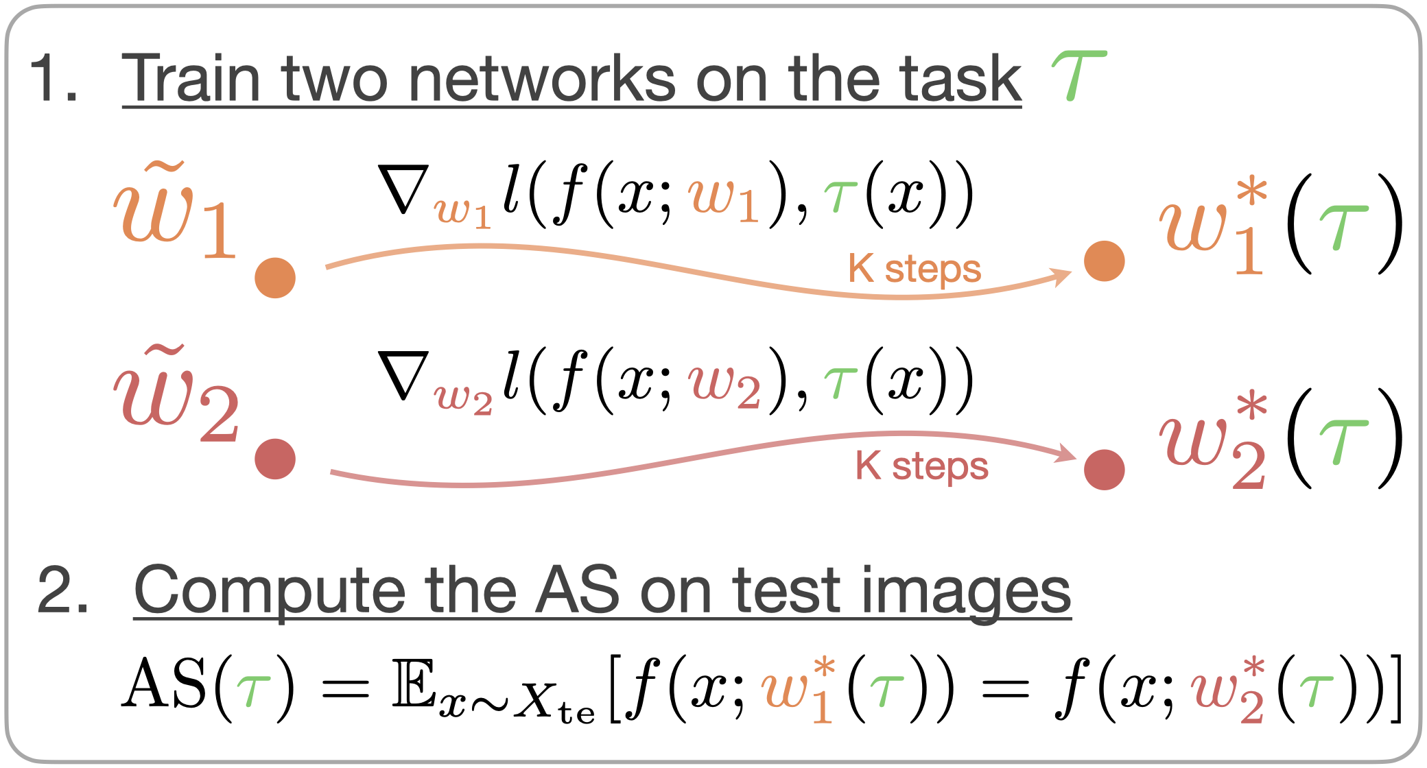
Agreeement Score computation for a given task \(\tau\).
We show that the AS is useful for measuring how well a model generalizes on a task in practice, and it differentiates between random- and human-labelled tasks. The AS can also be seen in the context of bias-variance decomposition, where it estimates the variance term of the test error. Please see our paper for a more detailed discussion on the connection between the AS and test accuracy (i.e., generalization). See below how the AS for random- and human-labelled tasks on CIFAR-10 images is distributed for different architectures.
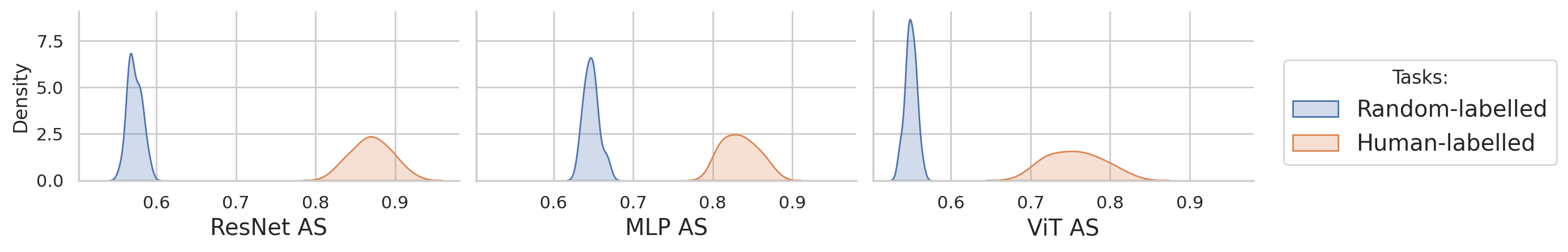
Agreemnt score for different tasks and architectures. The Agreement score differentiates semantic human-labelled tasks (high AS) from random-labelled tasks (low AS) across different architectures.
Task Discovery via Agreeement Score Meta-Optimization
As we saw above, the agreement score provides a good measure of generalization and distinguishes between human-labelled and random-labelled tasks. A natural question then arises:
Are there high-AS tasks other than human-labelled ones and what are they?
We approach this question empirically and introduce task discovery, a framework that finds high-AS tasks automatically by optimizing the AS over the space of all tasks.
Task Space Parametrization
Having tasks parametrized by discrete label assignment results in an expensive discrete optimization problem. We, therefore, suggest a continuous parametrization of the space of tasks to enable using more efficient first-order optimization methods. To do so, we model a task with a taks network \(t_\theta: X \to [0, 1]\) with parameters \(\theta \in \mathbb{R}^D\):
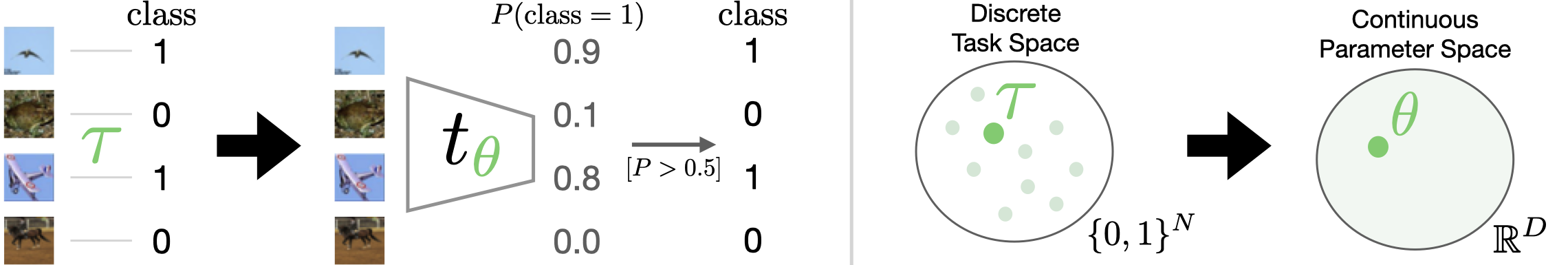
Task space parametrization.
Left: instead of modelling a task as a discrete label assignment, we parametrize it with a task network which outputs soft labels
, i.e., probability of class 1.
After that, we apply a thresholding function to get hard labels
corresponding to the task.
Right: this parametrization allows us to switch from the discrete task space to continous parameters space for optimization.
Note that we do so only for optimization and use the hard labels as the final task.
Agreement Score Meta-Optimization
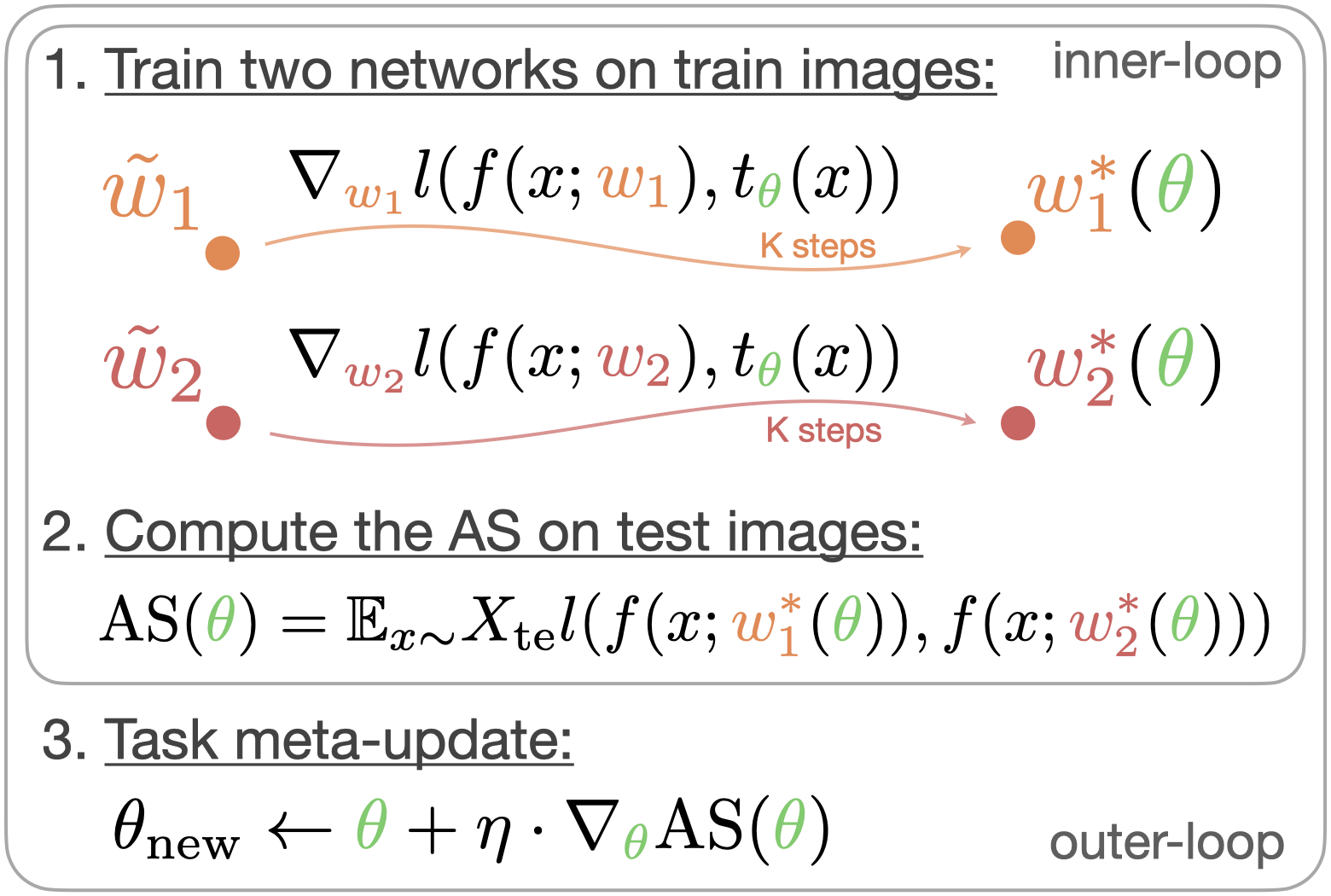
AS meta-optimization algorithm and exemplar vizualization. Agreement score meta-optimization w.r.t. the task parameters \(\textcolor{#6ACC64}{\theta}\) consists of two loops of optimization. Inner-loop: given a task \(t_{\textcolor{#6ACC64}{\theta}}\), two networks with randomly-initialized parameters \({\textcolor{#EE854A}{\tilde{w_1}}}, \textcolor{#D65F5F}{\tilde{w_2}}\) are optimized with the cross-entropy loss \(l\) using training images labelled by the task. After training, the agreement between two networks is calculated on the test images \(X_{\mathrm{te}}\). Outer-loop: the task parameters \(\textcolor{#6ACC64}{\theta}\) are updated using the meta-gradient of the AS. Video: an example of a meta-optimization dynamic. The task starts from a low-AS random-labelled one and converges to a high-AS task.
Discovering a Set of Dissimilar Tasks
The described meta-optimization process results only in a single task with a high AS. However, there are (potentially) many high-AS tasks. We therefore, aim to find a set of high-AS tasks \(T = \{t_{\theta_1}, \dots, t_{\theta_K}\}\). To do so, we additionally introduce a similarity loss to find sufficiently different tasks, resulting in the following optimization problem: \[ \arg\max_{T = \{t_{\theta_1}, \dots, t_{\theta_K}\}} \mathbb{E}_{t_{\theta} \sim T} AS(t_{\theta}) - \lambda \cdot L_{\mathrm{sim}}(T), \] where \(\lambda\) controls for the trade-off between how similar the tasks are and how high the average AS is (see the Appendix for more details on this trade-off). As modelling the set of tasks \(T\) with \(K\) separate task networks is memory and computationally inefficient, we suggest an amortize approach where all the tasks share the same encoder and differ in the last linear layer. See Section 4.3 of the paper for more details on how we model the set of task with a shared embedding space and how does the similarity loss \(L_{\mathrm{sim}}\) look in this case.
Vizualization of the Discovered Tasks
The task discovery framework outlined above allows finding multiple tasks that have a high AS on par with human-labelled ones, as can be seen from the plot below. Further, we show examples of different high-AS tasks discovered for the ResNet-18 architecture.
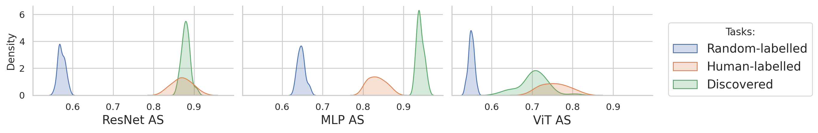
AS for random-labelled, human-labelled, and discovered task on CIFAR-10 images.
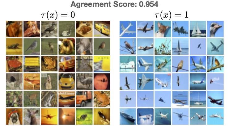
Discovered tasks on CIFAR-10 images for ResNet-18
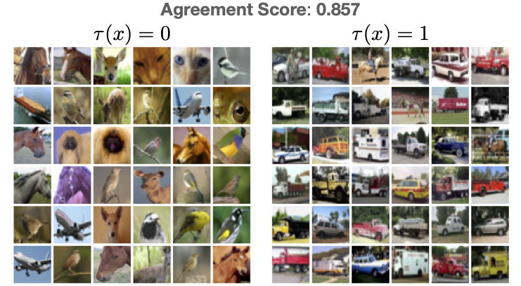
Below, we show examples of tasks discovered on CIFAR-10 images for the ResNet-18 architecture. For each task, we show exemplar images from both classes. We choose images with the highest probability for the corresponding class to show the most representative ones. Use and to switch between different tasks. We also provide additional images not shown on the right for the quiz. Use 0/1 buttons to make your prediction according to the task vizualization on the left and the eval button to evaluate your preddictions.
Task Vizualization
Test Examples: Quiz
Regulated task discovery
The standard (unregulated) task discovery can find any task that a given network generalizes on, resulting in discovering any tasks with a high AS. It might be desired, however, to guide task discovery to find particular tasks. To do this, we introduce a regulated task discovery framework. In the general case, the regulation can be achieved by adding additional objectives to the optimization that favour one tasks over the others, or confining the set of possible tasks (e.g., by changing the architecture of the task network). Here, we show an example of regulated task discovery using contrastive SimCLR pre-training for the task encoder. This way, we regulate the discovery process to find only those tasks invariant to the set of augmentations used in SimCLR. For example, since the colour-jitter augmentation is used during pre-training, the discovered tasks seem less colour-based and more semantic-based.
Task Vizualization
Test Examples: Quiz
Use buttons below to explore different discovered tasks.
Discovered tasks that are hard to interpret
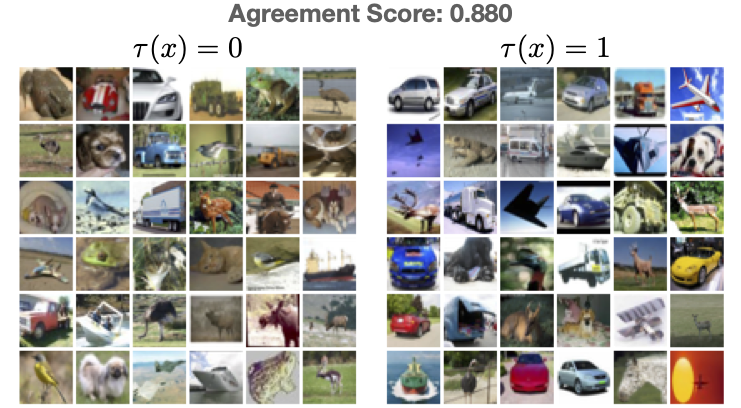
It was probably relatively easy to understand the pattern behind the tasks shown above and make a correct prediction with accuracy better than the chance level of 0.5. This suggests that these tasks are human-interpretable, i.e., can be easily understood and learnt by humans visually. Try now to understand the pattern behind these discovered tasks we show below, which also have a high AS!
Task Vizualization
Test Examples: Quiz
Use buttons below to explore different discovered tasks.
Was it more challenging this time? It was probably hard to achieve accuracy better than the chance level this time, i.e., these tasks are not human-interpretable. This is expected as task discovery is only concerned with finding high-AS tasks on which the network can generalize, and not all of them have to be visually interpretable by humans. The network (ResNet-18, in this case) can learn the pattern and generalize to novel images, as seen by the high AS of around 0.88. See the paper for a more in-depth discussion on human-interpretability.
Adversarial splits
The discovered tasks reflect inductive biases of a given network and statistical patterns in the data. We now show how they can be used to highlight the network's failure modes.
When training a network on a target task of interest (e.g., a human-labelled one), we usually split the dataset randomly into train and test sets to evaluate the performance. We show how to use discovered tasks to construct adversarial train-test splits, s.t., after training on the train set, the network fails on the corresponding test set.
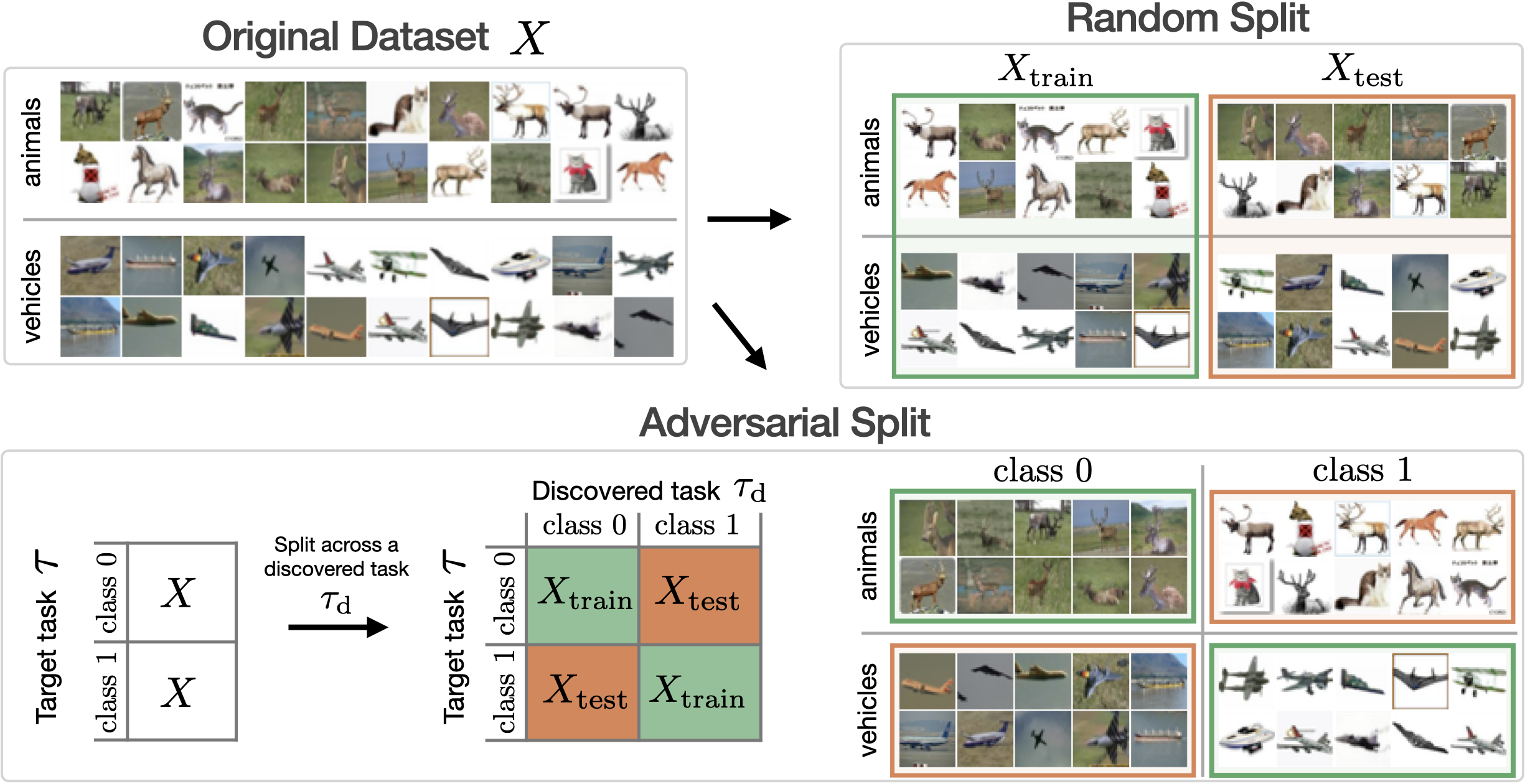
To construct an adversarial train-test split for a target task \(\tau\) (e.g., animals vs vehicles), we use a high-AS discovered task \(\tau_\mathrm{d}\). We induce a correltaion between them by putting images for which \(\tau_\mathrm{d}(x) = \tau(x) \) to the train set and the rest to the test set. Refer to the paper to see how this idea can be easily extended to create adversarial splits for multi-class classification tasks.
We found that when trained and tested on the adversarial split, the network's test performance drops significantly compared to a random train-test split as can be seen below for different datasets.
| Split | CIFAR-10 2-way tasks |
CIFAR-10 10-way |
ImageNet 1000-way |
CelebA 2-way |
|---|---|---|---|---|
| Random | 0.81 ± 0.03 | 0.78 ± 0.04 | 0.59 ± 0.01 | 0.94 ± 0.00 |
| Adversarial | 0.17 ± 0.04 | 0.41 ± 0.10 | 0.42 ± 0.02 | 0.29 ± 0.00 |
The discovered task \(\tau_\mathrm{d}\), in the case of adversarial split, can be seen as a spurious feature, and the adversarial split creates a spurious correlation between \(\tau\) and \(\tau_\mathrm{d}\), that fools the network. Similar behaviour was observed before on datasets where spurious correlations were curated manually (e.g., WILDS benchmark). In contrast, the described approach using the discovered tasks allows us to find such spurious features to which networks are vulnerable, automatically. It can find spurious correlations on datasets where none was known to exist (as in CIFAR-10 and ImageNet examples) or find new ones on existing benchmarks as we show for CelebA in the paper. See visualization of different adversarial splits below.
CIFAR-10 adversarial splits
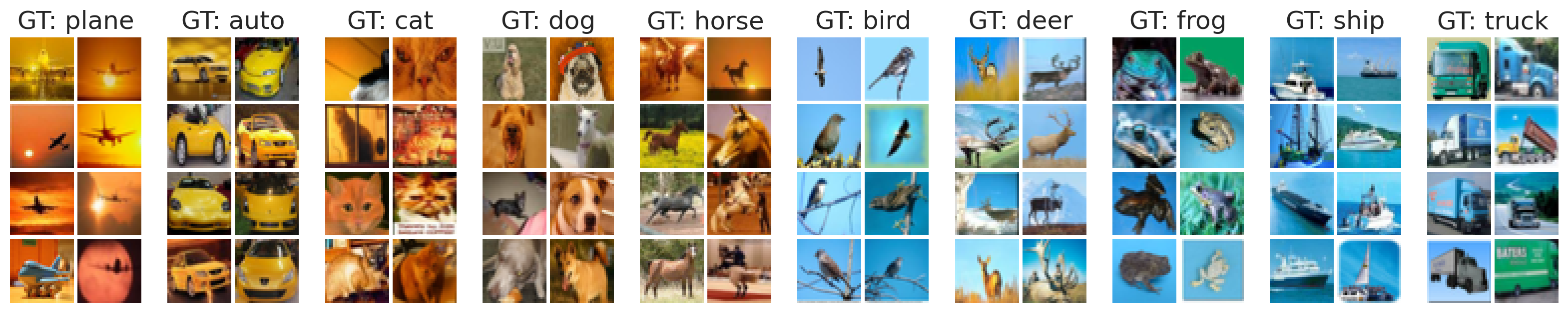
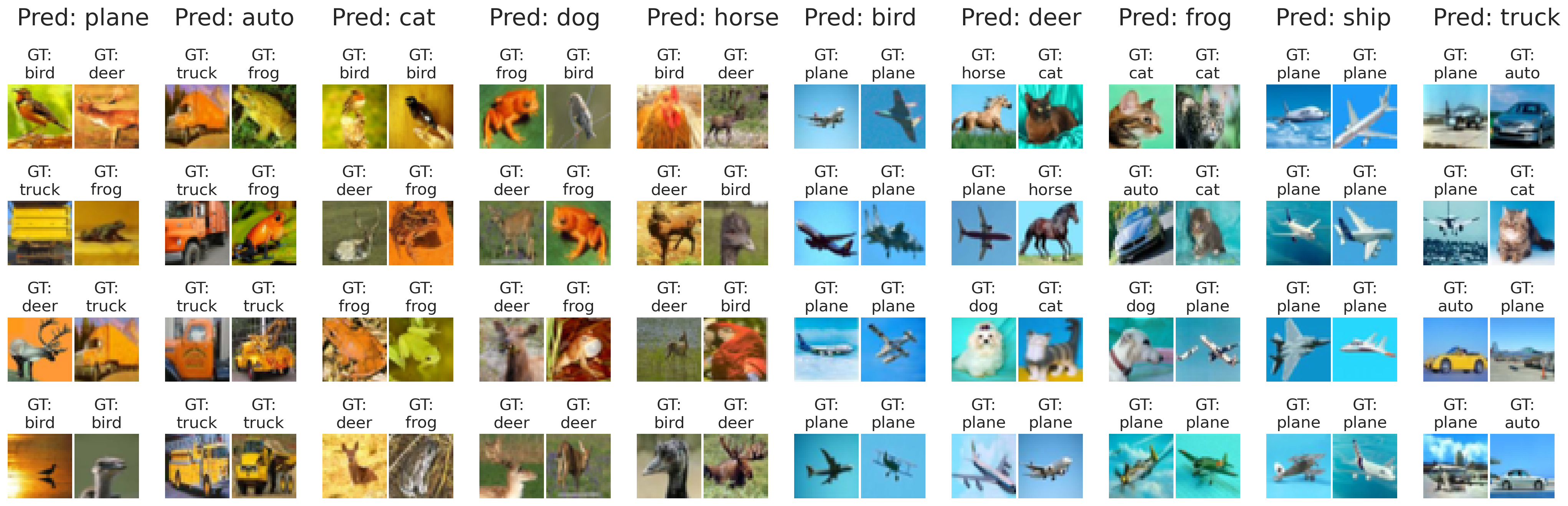
Below we show multiple adversarial splits for the CIFAR-10 dataset based on different discovered tasks with high AS. Use and buttons to switch between different adversarial splits. For test images, each column corresponds to ground truth classes, and the network's prediction (Pred) is shown on top of each image. For mistaken (test) images, each column corresponds to classes predicted by the network, and the ground truth class (GT) is shown on top of each image. Note how the network confuses test examples in accordance with the pattern represented by the discovered task used to create the adversarial split. For example in the first split, images from the first five classes appear yellowish and from the last five bluish.
Train
Test
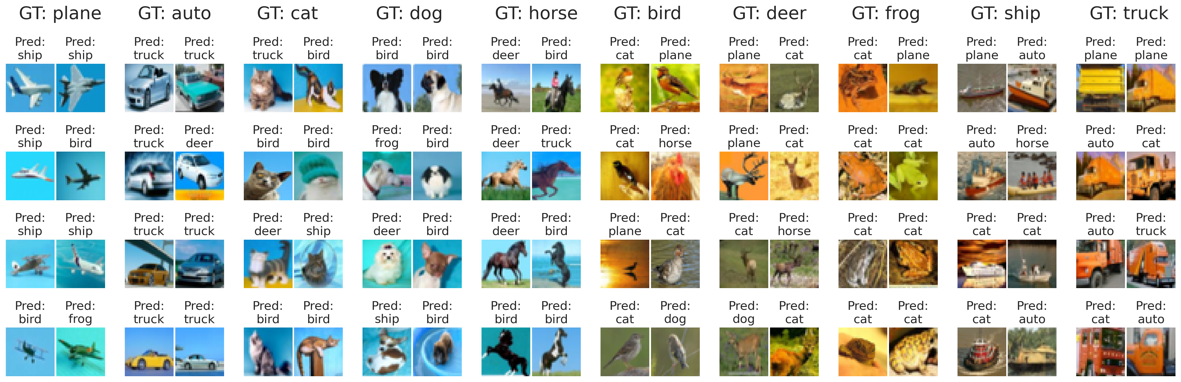
Mistakes
Use buttons below to explore different adversarial splits.
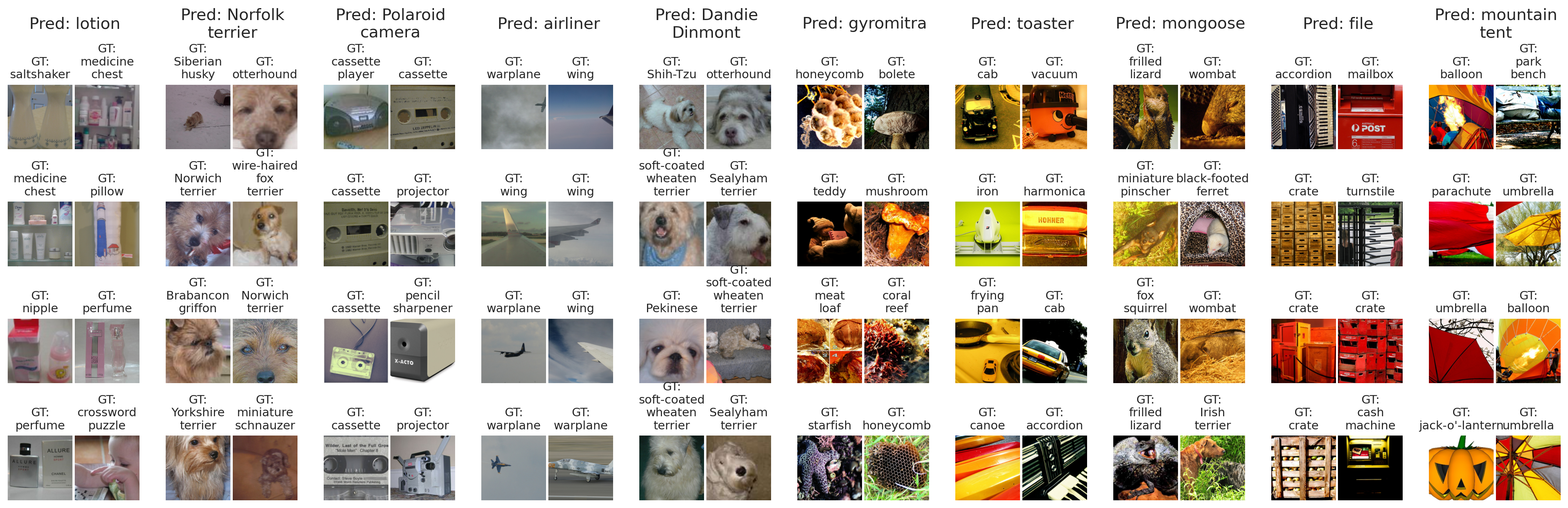
An ImageNet adversarial split
Below is an example of an adversarial split for the ImageNet dataset. We show a single split here, and you can use and buttons to switch between different classes. Similarly to the previous example, columns for test images correspond to ground truth classes, and for mistaken images, columns correspond to the network's prediction.
Train
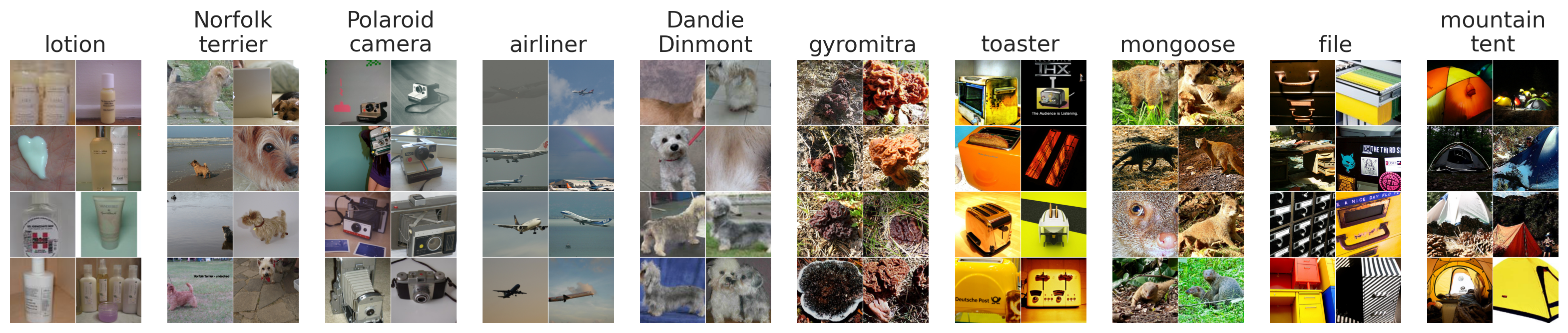
Test
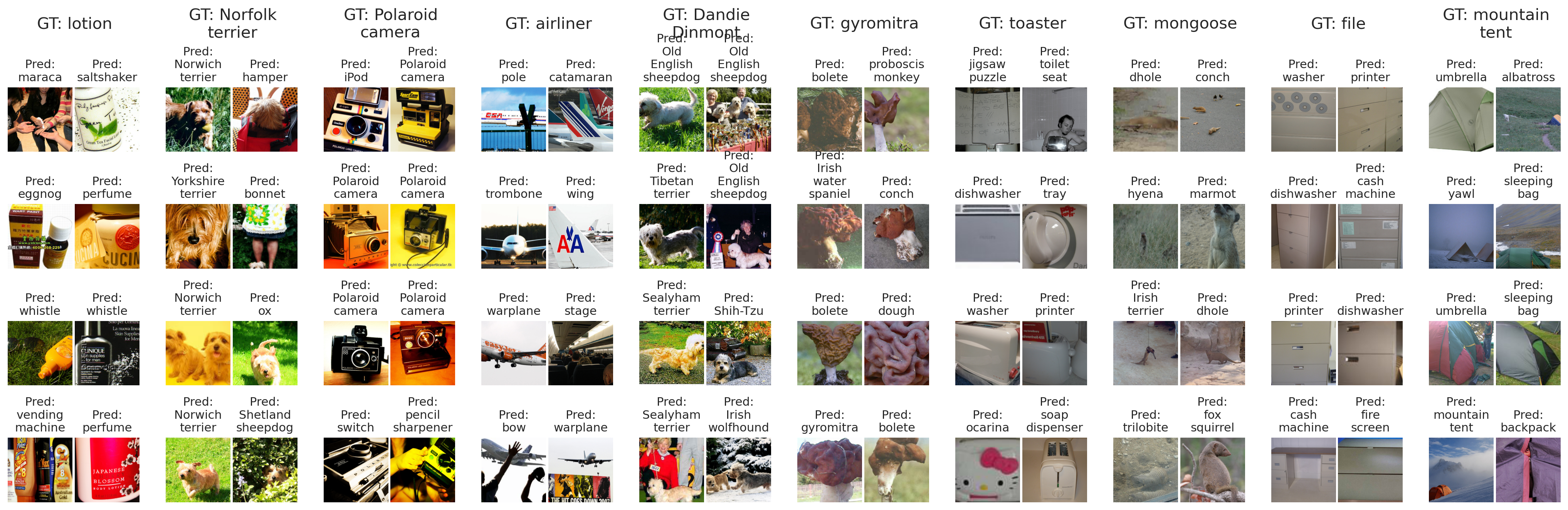
Mistakes
Use buttons below to explore different classes in the adversarial split.
BibTeX
@article{atanov2022task,
  author    = {Atanov, Andrei and Filatov, Andrei and Yeo, Teresa and Sohmshetty, Ajay and Zamir, Amir},
  title     = {Task Discovery: Finding the Tasks that Neural Networks Generalize on},
  journal   = {Advances in Neural Information Processing Systems},
  year      = {2022},
}